Monopoly Demand Curve
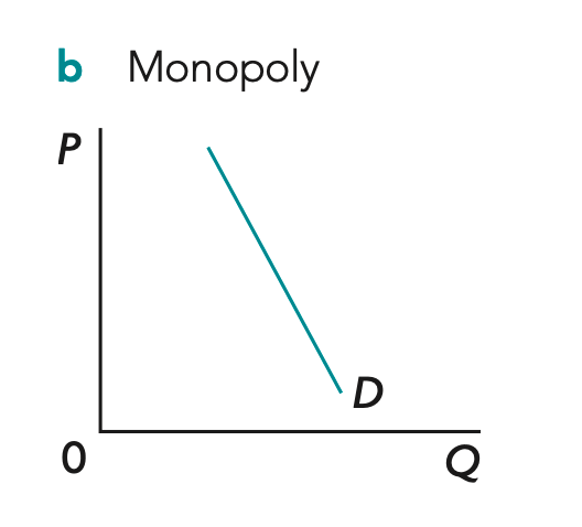
Diagram Explanation:
-
Monopoly = one firm, high barriers of entry
-
Firm is the entire industry -> so the monopoly’s demand curve is the market demand curve -> market demand is downward sloping -> at a high price, consumers demand a small quantity -> to sell a larger quantity, the monopoly must lower its price -> as output increases, price falls
-
Therefore, the monopoly faces a downward-sloping demand curve (D = AR)
Profit maximisation & loss minimisation in monopoly
Abnormal profit

-
The mkt price is Pe -> firm is a price maker so demand is downward-sloping (D=AR) -> firm chooses the profit maximizing output where MR=MC at Qe -> firm charges the highest price consumers are willing to pay for Qe on the demand curve which is Pe -> at Qe the AR (price) > AC -> so total revenue (AR × Q) > total cost (AC × Q)
-
The shaded area = abnormal profits earned by firm
-
The firm earns profits above the normal level because barriers to entry prevent new firms from entering the market
Diagram Explanation:
Normal profit
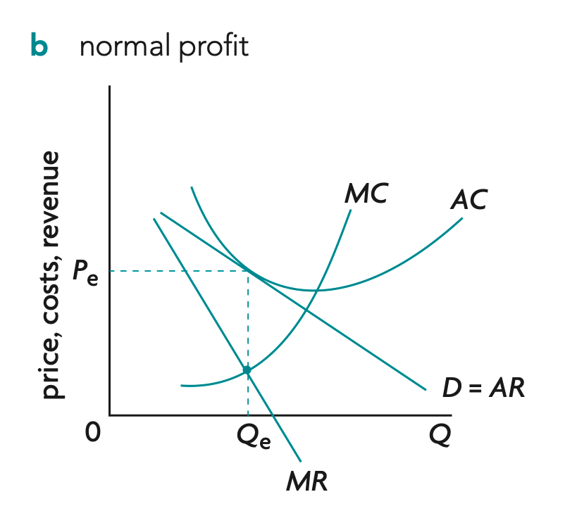
Diagram Explanation:
-
The mkt price is Pe -> firm is a price maker so demand is downward-sloping (D=AR) -> firm chooses the profit maximizing output where MR=MC at Qe -> firm charges the highest price consumers are willing to pay for Qe on the demand curve which is Pe -> at Qe the AR (price) = AC -> so total revenue (AR × Q) = total cost (AC × Q)
-
The firm earns normal profit
Loss
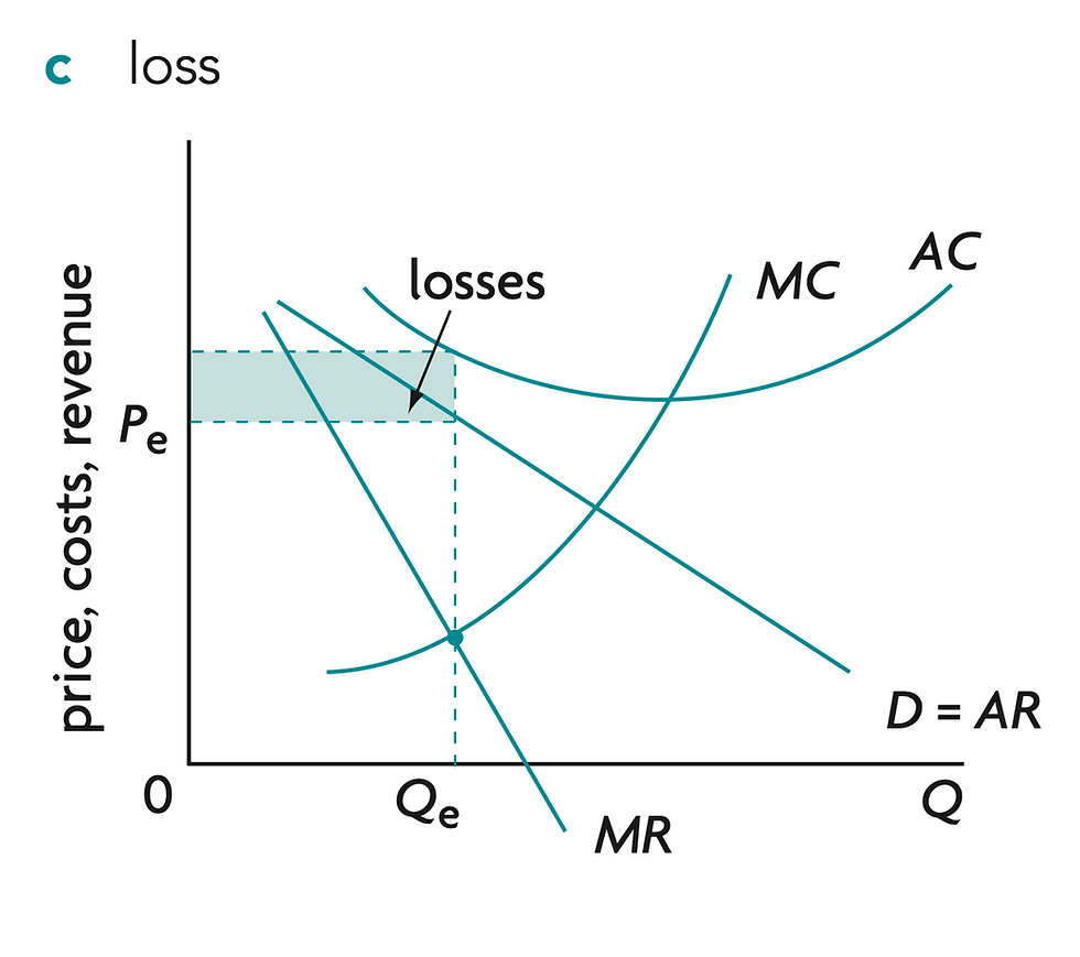
Diagram Explanation:
-
The mkt price is Pe -> firm is a price maker so demand is downward-sloping (D=AR) -> firm chooses the profit maximizing output where MR=MC at Qe -> firm charges the highest price consumers are willing to pay for Qe on the demand curve which is Pe -> at Qe the AR (price) < AC -> so total revenue (AR × Q) < total cost (AC × Q)
-
The shaded area = loss of the firm's revenue & profit
Natural monopoly
Diagram Explanation:
-
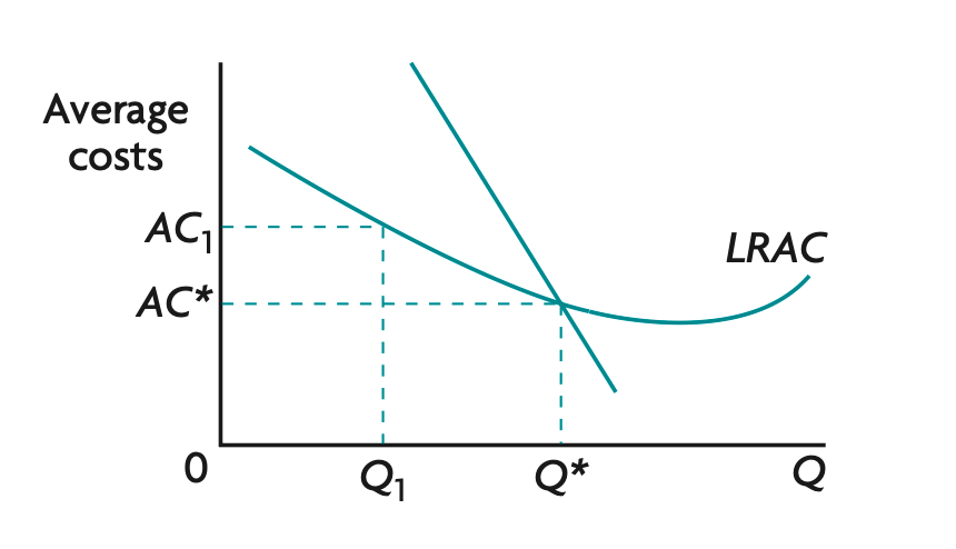
The firm increases its scale of production -> output increases from Q1 to Q* -> fixed costs are spread over more units and the firm benefits from economies of scale (e.g. specialization, bulk buying, managerial efficiency) -> average cost (AC) falls from AC1 to AC* -> firm moves down the LRAC curve
-
At Q*, the firm reaches the minimum efficient scale where average cost is at or near its lowest level -> producing at a larger scale allows the firm to produce more efficiently -> lower average costs allow the firm to charge lower prices while remaining profitable -> firm becomes more cost competitive.
Consumer and producer surplus and welfare loss in monopoly compared with perfect competition

Diagram Explanation:
-
Perfect competition produces at Qpc where MB = MC
-
consumer surplus is Area A
-
producer surplus is Area B
-
-
As a result -> total welfare is maximized
-
However, a monopolist instead chooses MR = MC -> output falls to Qm & price rises to Pm -> consumers buy fewer units at a higher price -> consumer surplus falls from C+D+E+F to C -> area D is transferred from consumers to producers -> areas E + F represent mutually beneficial trades that no longer occur -> E and F areas become deadweight welfare loss -> total welfare decreases -> monopoly is allocatively inefficient